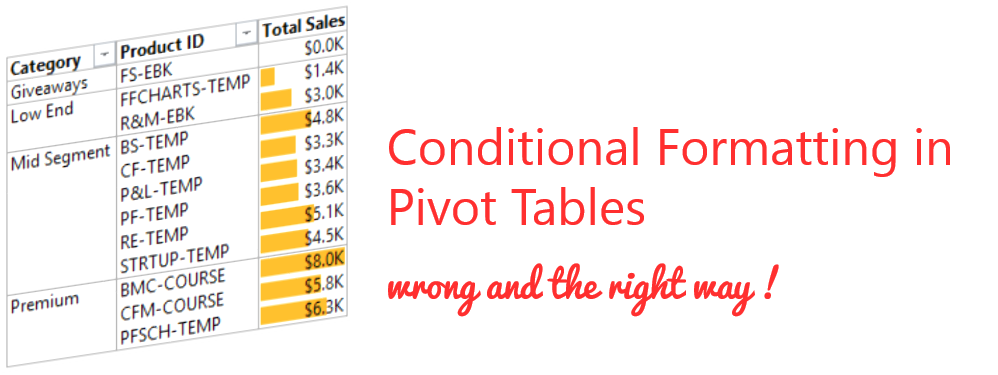
Today I am going to speak about a small problem that happens when you are trying to apply conditional formatting on Pivot Tables. It’s not complex rather its nifty!
Consider this Pivot Table..
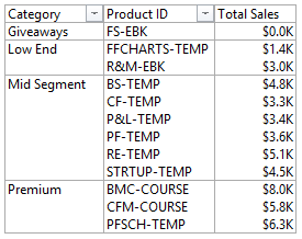
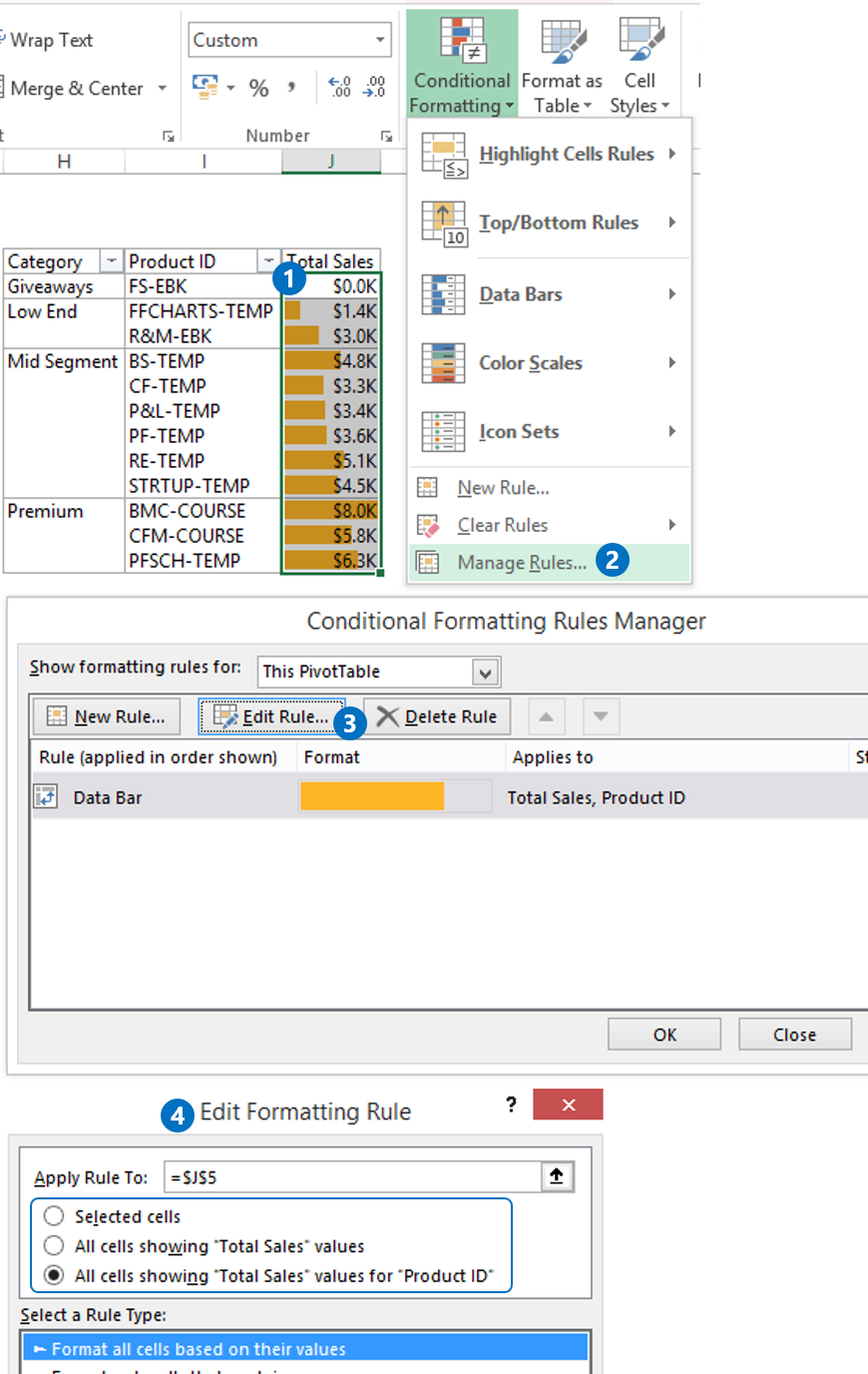
We have Product Category, Product ID and its Sales. What if I ask you to make it a little fancy and apply conditional formatting (data bars) on it ?
Applying Conditional Formatting on Pivot Tables – Wrong Way!
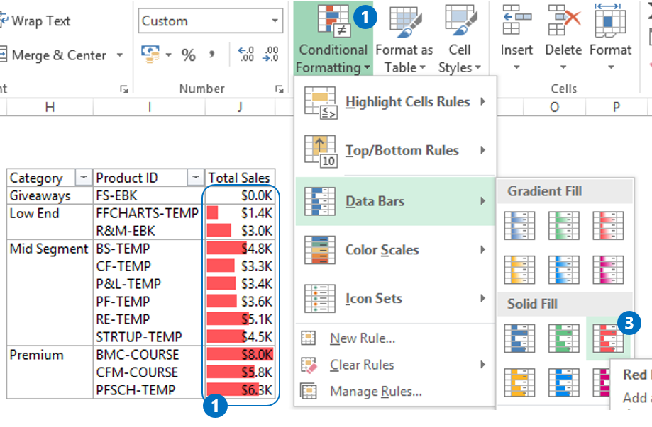
- Now if you selected the sales column of the Pivot Table
- Went to Conditional Formatting
- And applied a Data Bars on it
- That fine but the process isn’t complete yet and you are missing out on an additional step
Applying Conditional Formatting on Pivot Tables – Right Way!
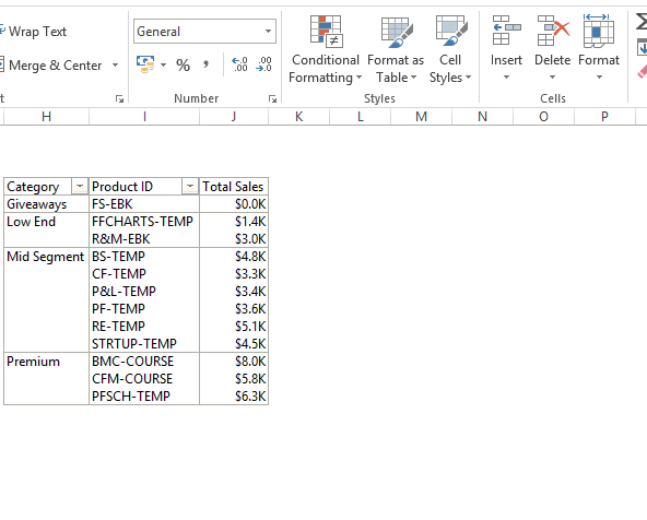
- Select the sales column of the Pivot Table
- Conditional Formatting
- Apply Data Bars on it
- Don’t forget to – Click the little icon at the bottom of the data selected and apply the formatting rule to the Pivot Fields
What difference does it make?
- If you don’t do the last step – Conditional Formatting is applied on the cells selected rather than on Pivot Table Fields
- In case your pivot table structure changes, your formatting will go for a toss. Because your formatting was applied to the cells and not to the Pivot Table Fields
Little Nuances!
- You might have noticed that there were 3 options available when you clicked on the drop down for applying conditional formatting to the pivot table. Here is what they mean!
- Selected Cells – Will apply the formatting to selected cells only
- All cells showing “Total Sales” values – Conditional Formatting will be applied to Total Sales irrespective of the pivot table structure. For eg – As of now we have Category, Product ID and Sales, even if you remove the Product ID from the pivot, the formatting will remain intact on the sales
- All cells showing “Total Sales” values for “Product ID” – If you remove product ID from the Pivot, the formatting on sales will disappear. Because the formatting is applied on “Sales for Product ID” and not the standalone “Sales” Field
- This option will appear for all the built in Conditional Formatting features (Highlight Cells, Top Bottom Rules, Colors, Data Bars, Icons etc..) when applied on the Pivot Table
- Just in case you lose the drop down, you can still change the formatting options from the Edit Rule Dialogue box
Which method do you use?
Have you been using the conditional formatting correctly? Let me know in the comments